
Edge detection is a major component of image processing. Despite multiple advances in deep-learning-based techniques such as Convolutional Neural Networks that can perform very complex edge detection (i.e. edges with varying curvature, noise, color etc.), classical edge detection methods are still highly relevant in certain cases! An example would be if the data is known to be simple and predictable; a Canny Edge Detector would work right out of the box compared to a CNN which typically is more complicated to implement.
Edge Detection Basics
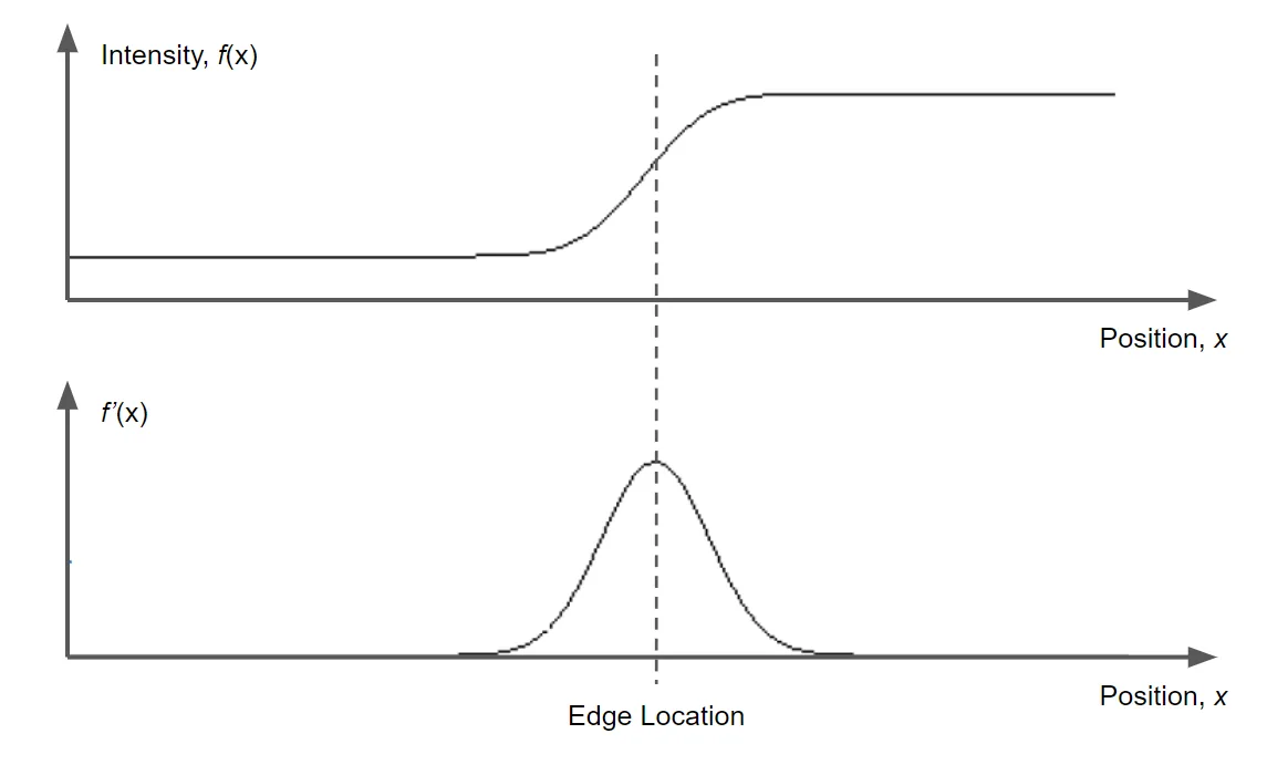
Most classical edge detection algorithms are based on the concept of first derivatives. In the figure below, we see a theoretical edge profile, with the y axis being pixel intensity and x axis being the physical location in an image. At an edge location in an image, there is a quick transition from low to high intensity or vice-versa. The faster this transition, the sharper the edge will appear. To detect the edge, we simply take the first derivative of the pixel intensities, and look for the maximum points as seen in the second graph below!
Canny Edge Detector
Usually, this derivative is combined with a Gaussian filter in order to perform image-smoothing and edge detection in one step. Since the derivative and Gaussian filter convolution are linear operations, we simply apply the differentiated Gaussian filter directly to the image! Below shows a sample 5x5 filter that completes this operation, with σ = 1.
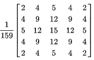
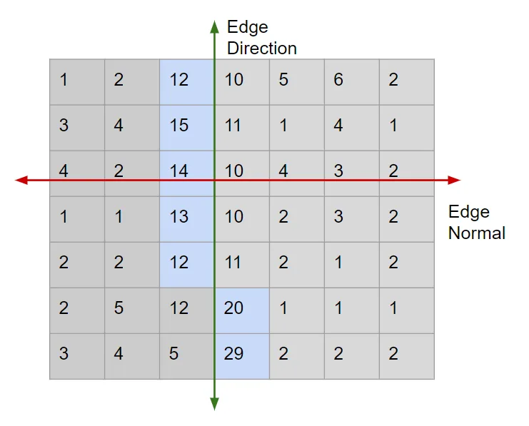
This produces an output that already highlights the position of edges with a high value! However, the advantage of Canny is that it produces very thin and clean edges. The next step, non-maximum suppression (NMS) will achieve this. NMS is done by tracking along the high values in the output image, then checking for maximal gradients in a 3x3 neighborhood. The center pixel has to be the highest in the direction perpendicular to the edge, or else it will be set to 0.
In the example below, we see a 7x7 matrix with sample outputs from the Gaussian filter. High values will indicate that the first derivative is high at that location! To perform NMS, we track along the edge direction, then set values to 0 if they are not the maximum in the edge normal direction (i.e. red axis). Therefore, the blue cells will remain and the gray cells will all be set to 0 after NMS. We see that this gives a fine edge output that is only one pixel wide!
Another crucial component of Canny Edge detection is hysteresis thresholding. This sounds super complicated, but it is pretty straightforward! This step is performed in tandem with NMS, and the main idea is to prevent noisy edges from causing fragmentation in the final edge detection. Two threshold values are selected, with T1 > T2. The NMS tracking only starts if the gradient values are higher than T1, and stop only if gradient values are lower than T2. This ensures that NMS tracking has some robustness to noisiness in the edges, where this tolerance can be controlled by the T1 and T2 values.
Conclusion
Though Canny Edge detectors and the various classical edge detection methods might seem overshadowed by the ever-popular CNNs and Deep Learning methods, we should not forget their simplicity and effectiveness. Sometimes it is much easier to try a classical solution, and it might work better than you expect!