Introduction to Squeeze-and-Excitation Networks

Squeeze-and-Excitation Networks (SENet) were the winners of the ImageNet Classification Challenge in 2017, surpassing the 2016 winners by a relative improvement of around 25%. SENets introduced a key architectural unit — Squeeze-and-Excitation Block (SE Block) which was crucial to the gains in performance. SE Blocks can also be easily added to other architectures with low additional overhead.

Introduction to SE Blocks

Typically, CNNs work by extracting information from the spatial dimensions and storing them in the channel dimensions. This is why the spatial dimensions of feature maps shrink while the channels grow as we go deeper in a CNN. All channels are weighted equally when considering the output feature map of one particular CNN layer.

Earlier CNN layers tend to capture basic features such as edges, corners, and lines, while later layers capture higher-level features such as faces and text.

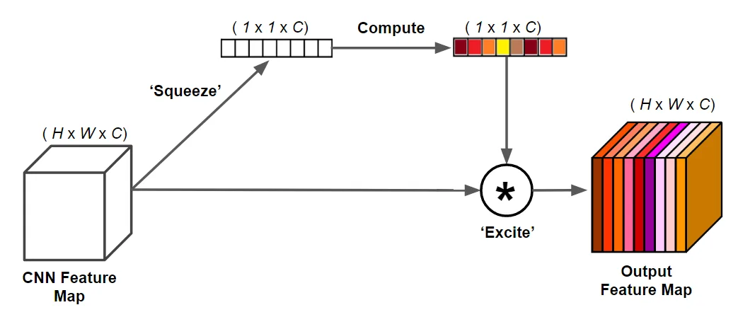
The main idea of an SE block is to assign each channel of a feature map a different weight (excitation) based on how important that channel is (squeeze).

Technical explanation

SE blocks can be split into three main parts: squeeze, computation, and excitation.

1. Squeeze. Global Average Pooling is performed on the output feature map of the CNN layer. This is essentially taking the average value over all activations in the spatial dimension (H x W), giving one activation per-channel. The result of this is a vector of shape (1 x 1 x C).
2. Computation. Vector from the previous operation is passed through two successive Fully-Connected Layers. This serves the purpose of fully capturing channel-wise dependencies that were aggregated from the spatial maps. A ReLU activation is performed after the first FC layer, while the sigmoid activation is used after the second FC layer. In the paper, there is also a reduction ratio such that the intermediate output of the first FC layer is of a smaller dimension. The final output of this step also has a shape (1 x 1 x C).
3. Excitation. Lastly, the output of the computation step is used as a per-channel weight modulation vector. It is simply multiplied with the original input feature map of size ( H x W x C ). This scales the spatial maps for each channel according to their ‘importance’.

SE Blocks can be easily integrated with many existing CNNs. In the paper, architectures such as ResNets, VGG and Inception had their accuracy boosted significantly, yet at a low additional computational cost.

Code Example

Here is a sample code snippet that you can experiment with. Written in PyTorch. As you can see, it is really simple to add in the functionality of Squeeze-and-Excitation blocks! In about 10 lines of code, we have a modular implementation from moskomule that can be easily implemented to most Deep CNNs.

class SELayer(nn.Module):
    def __init__(self, channel, reduction=16):
        super(SELayer, self).__init__()
        self.avg_pool = nn.AdaptiveAvgPool2d(1)
        self.fc = nn.Sequential(
            nn.Linear(channel, channel // reduction, bias=False),
            nn.ReLU(inplace=True),
            nn.Linear(channel // reduction, channel, bias=False),
            nn.Sigmoid()
        )

def forward(self, x):
    b, c, _, _ = x.size()
    y = self.avg_pool(x).view(b, c)
    y = self.fc(y).view(b, c, 1, 1)
    return x * y.expand_as(x)

Conclusion

The main appeal of SE Blocks would be their simplicity. Just from the figure alone, we can understand the functionality and steps involved in the Squeeze-Excite process. Furthermore, they can be added into models without much increase in computational cost, so everyone should experiment with integrating this into their deep learning architectures!

References

• Squeeze-and-Excitation Networks
• PyTorch
• moskomule/senet.pytorch

← Back to the blog